ERROR
PROPAGATION
1. Measurement of Physical Properties
The value of a physical property often depends on one or more measured quantities
![]()
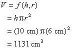
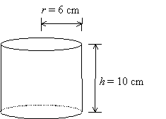
Example: Volume of a cylinder
|
|
|
|
2. Systematic Errors
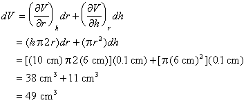
A systematic error in the measurement of x, y, or z leads to an error in the determination of u.

This is simply the multi-dimensional definition of slope. It describes how changes in u depend on changes in x, y, and z.
Example: A miscalibrated ruler results in a systematic error in length measurements. The values of r and h must be changed by +0.1 cm.
|
|
|
3. Random Errors
Random errors in the measurement of x, y, or z also lead to error in the determination of u. However, since random errors can be both positive and negative, one should examine (du)2 rather than du.

If the measured variables are independent (non-correlated), then the cross-terms average to zero
![]()
as dx, dy, and dz each take on both positive and negative values.
Thus,

Equating standard deviation with differential, i.e.,
![]()
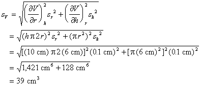
results in the famous error propagation formula
|
|
This expression will be used in the Uncertainty Analysis section of every Physical Chemistry laboratory report!
Example: There is 0.1 cm uncertainty in the ruler used to measure r and h.
|
|
|
Thus, the expected uncertainty in V is ±39 cm3.
4. Purpose of Error Propagation
· Quantifies precision of results
|
|
Example: V = 1131 ± 39 cm3 |
· Identifies principle source of error and suggests improvement
|
|
Example: Determine r better (not h!) |
· Justifies observed standard deviation
|
|
If sobserved » scalculated then the observed standard deviation is accounted for If sobserved differs significantly from scalculated then perhaps unrealistic values were chosen for sx, sy, and sz. |
· Identifies type of error
|
|
If ½uobserrved - uliterature½ £ scalculated then error is random error If ½uobserrved - uliterature½ >> scalculated then error is systematic error |
5. Calculating and Reporting Values when using
Error Propagation
Use full precision (keep extra significant figures and do not round) until the end of a calculation. Then keep two significant figures for the uncertainty and match precision for the value.
Example: V = 1131 ± 39 cm3
6. Comparison of Error Propagation to
Significant Figures
Use of significant figures in calculations is a rough estimate of error propagation.
|
Example: |
|
Keeping two significant figures in this example implies a result of V = 1100 ± 100 cm3, which is much less precise than the result of V = 1131 ± 39 cm3 derived by error propagation.
7. Common Applications of the Error Propagation
Formula
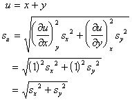
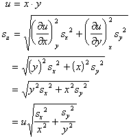
Several applications of the error propagation formula are regularly used in Analytical Chemistry.
|
Example: |
|
|
Example: |
|
Analytical chemists tend to remember these common error propagation results, as they encounter them frequently during repetitive measurements. Physical chemists tend to remember the one general formula that can be applied to any case, as they encounter widely varying applications of error propagation. (Or perhaps analytical chemists take a more utilitarian approach, whereas physical chemists take a more "from first principles" approach.)
